
How Sensor Feedback Enables Accurate Variable-Rate Fertilization in Field Conditions
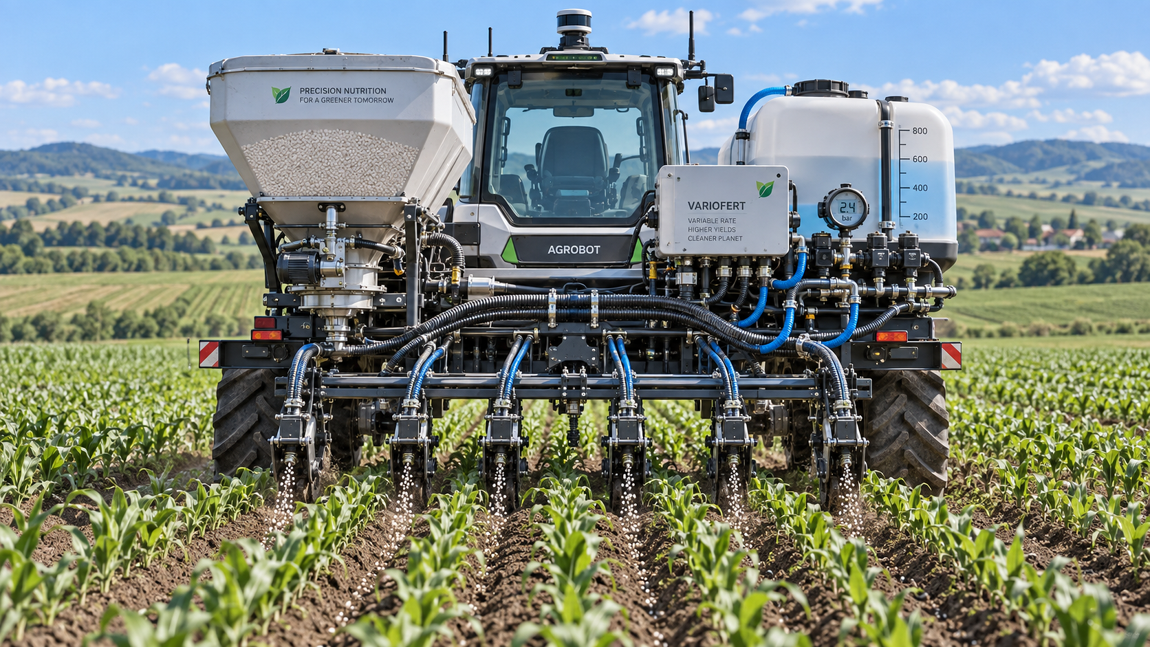




Accurate variable-rate fertilization is achieved when the commanded rate, the material actually delivered, and the agronomic condition at a specific field location remain aligned while the machine is moving. A prescription map supplies an intended rate, but it cannot confirm whether a spreader, planter-mounted applicator, or liquid toolbar is meeting that command after speed changes, product bridging, pressure fluctuations, slope transitions, or sensor drift. Sensor feedback closes that gap by turning a planned application into a monitored control process.
For precision fertilization systems with sensor feedback, the central technical question is straightforward: which measurement represents the condition that needs correction, and how quickly can the controller act before the machine has traveled beyond the affected area? A system can have accurate positioning and a detailed prescription while still applying the wrong mass per hectare if the delivery path is not measured and controlled under field load.
Rate accuracy begins with the distinction between command and delivery
A variable-rate controller commonly calculates a target mass or volume from location, prescription zone, machine width, and forward speed. That target is transmitted to a metering drive, valve, pump, gate, conveyor, or spinner-disc feed system. The calculation is only the first part of rate control. The physical material flow can diverge from the command for reasons that are not visible in the prescription layer.
Granular fertilizer is particularly sensitive to flow-path behavior. Product density, granule size distribution, moisture uptake, dust content, hopper angle, agitator action, and gate geometry all influence how much material reaches the metering element. A setting that produced the expected flow at the edge of a field may behave differently after vibration compacts material in the hopper or after a humid product begins to bridge. Liquid fertilizer has different failure modes: pump wear, filter restriction, air entrainment, changing tank head, nozzle wear, and pressure loss across section plumbing can alter delivery.
Feedback sensors distinguish a controller that assumes output from one that verifies output. A shaft encoder may confirm metering rotation, but rotation alone does not prove mass flow. A flowmeter can verify liquid movement, though its reading must be interpreted with regard to pulsation, viscosity, and placement in the plumbing circuit. Load cells beneath a hopper provide a direct mass-loss reference over time, but their signal is affected by terrain acceleration and cannot always support rapid, row-by-row correction without filtering. Each sensor therefore answers a different control question.
Sensor feedback has two separate jobs
Field systems often combine sensors without separating their roles. One set of sensors estimates where and how much nutrient is needed. Another set verifies whether the applicator delivered the commanded rate. Mixing these jobs can lead to misleading conclusions.
Soil electrical conductivity, apparent soil moisture, organic matter maps, soil sampling layers, terrain data, and crop reflectance may contribute to a rate decision. They represent spatial variability or a proxy for nutrient response. They do not establish applied-rate accuracy. Conversely, a highly accurate flowmeter can confirm liquid delivery but says nothing about whether the prescribed nitrogen rate matched crop demand.
The distinction becomes important when a treated strip appears underperforming. A crop sensor may indicate low vigor because the crop is water-limited, root-restricted, diseased, compacted, or genuinely nitrogen-deficient. A low reflectance value should not automatically trigger more fertilizer. Where crop sensing is used for on-the-go adjustment, its agronomic model needs guardrails based on growth stage, prior nutrient application, moisture condition, and zones where additional nutrient is unlikely to produce a response.
Likewise, an as-applied map showing a uniform commanded rate is not evidence of uniform placement. It records controller intent unless it is populated from measured delivery data and correctly time-aligned with machine position. A useful record identifies whether a rate value came from a target, an actuator estimate, a measured flow value, or a post-operation mass balance.
Latency determines whether closed-loop correction is spatially meaningful
Every variable-rate system has delay. Position data arrive after a measurement interval. The controller processes the target rate. The actuator responds. Material then travels from meter to outlet and, in some machines, through a long delivery tube or boom line. The applied fertilizer reaches the soil after the machine has moved forward. If these delays are not represented in controller setup, the system may apply the correct quantity in the wrong place.
Delay is especially visible at prescription boundaries. A sharp rise in commanded rate may appear downstream of the intended zone because product already in the delivery path continues to move. A decrease can leave an overdosed tail for the same reason. Granular pneumatic systems have transport delay that varies with hose length, air velocity, product characteristics, and blockage state. Liquid systems show delay from line volume, valve response, pump ramp rate, and recirculation arrangement. Spinner spreaders add a lateral distribution delay because granules take time to leave the disc and land across the working width.
Forward speed turns time delay into distance error. At a higher travel speed, the same mechanical response time covers more ground. This is why a controller that seems stable during a stationary calibration or a slow test pass can show poor zone alignment during normal operation. Speed feedback must therefore be reliable and sufficiently fast. GNSS-derived speed is often suitable, but signal quality, receiver configuration, update rate, and short-term motion on uneven terrain should be considered alongside wheel-based speed sensing. Wheel speed can be affected by slip; GNSS can be affected by delayed updates or poor correction availability. Comparing the two signals during operation can expose conditions that deserve attention.
Control tuning also matters. An aggressively tuned loop may chase noisy flow readings, repeatedly overshooting the target as pressure or metering speed changes. Excessive smoothing has the opposite problem: stable traces on a display but delayed correction in the field. The appropriate response depends on actuator capacity, product transport delay, expected prescription variability, and the spatial resolution that the crop-management decision can realistically support.
Application resolution must match machine dynamics
A prescription map may contain small polygons or tightly spaced grid values, yet the applicator cannot necessarily reproduce each transition. The effective resolution is limited by boom length, section width, travel speed, communication rate, metering response, and product residence time. Requesting rapid changes that are shorter than the delivery system's response distance produces a visually detailed map but a physically blurred application.
A practical evaluation compares prescription transition length with measured step response. During a controlled pass, command a known rate increase, record the actual flow or mass response, and measure the distance to stable delivery. Repeat at representative speeds and with fertilizer at the expected temperature and moisture condition. The resulting response distance provides a defensible basis for deciding whether rate zones need smoothing, larger management units, or different control parameters.
Granular and liquid systems require different evidence
Granular application is commonly assessed through both total mass and distribution pattern. A hopper load-cell system can show whether the machine consumed approximately the intended total mass over a pass. That is valuable, but it can conceal section-level or side-to-side error. A spreader might discharge the correct total quantity while producing an uneven transverse pattern because vane wear, disc speed, feed point, product trajectory, or crosswind altered the throw.
Catch-tray testing remains relevant for broadcast spreaders because it measures the pattern that reaches the ground. The result should be checked with the actual fertilizer formulation, not only with a generic calibration material. Granules that differ in size, shape, hardness, or bulk density can separate in flight and shift the effective spread pattern. The overlap behavior between adjacent passes matters as much as the pattern from one pass. A rate controller cannot correct a poor distribution pattern simply by changing the total feed rate.
For liquid systems, a single main-line flowmeter may confirm total boom output while hiding unequal delivery among sections or rows. Pressure differences caused by hose length, fittings, elevation, partially restricted strainers, or worn nozzles can create local variation. Section flow sensing, nozzle-level monitoring, or periodic nozzle output tests reveal whether the total measured flow is being distributed as intended. When liquid fertilizer concentration changes between batches, volumetric flow should be converted carefully if the agronomic prescription is defined by nutrient mass rather than product volume.
Terrain and machine motion complicate apparently simple measurements
Field feedback signals are rarely clean. Load cells react to vertical acceleration, side loads, frame flex, and turning forces. A sloped pass may change the mechanical load path through a hopper frame. Pressure sensors show transients when sections open or close. Optical crop sensors respond to shadow, soil background, row spacing, crop residue, and sensor-to-canopy distance. Treating every short fluctuation as a true agronomic or delivery event produces unstable control.
Filtering is necessary, but it should be tied to the purpose of the measurement. A load-cell signal used for end-of-pass mass reconciliation can be smoothed heavily because it is not controlling a rapid actuator response. A signal used to detect a sudden blockage needs enough responsiveness to identify a meaningful deviation before a large untreated area develops. Filtering settings should be documented with the sensor location and the action they trigger; otherwise, a later review cannot distinguish a real delivery issue from a deliberately filtered signal.
Turns, headlands, and section transitions deserve separate attention. Many systems suppress rate control or alter their logic during low-speed turns. That behavior can be appropriate, but it changes how coverage and applied mass are represented in records. Overlap control also depends on accurate implement geometry. Incorrect antenna-to-application-point offsets shift section shutoff and rate transitions even when the GNSS position itself is accurate.
Calibration is a chain, not a single machine setting
Calibration begins with the fertilizer product and ends with the applied record. For granular material, a calibration factor established with dry, free-flowing product may become invalid after storage conditions change. For liquid material, flowmeter calibration should account for the relevant fluid rather than assuming water-based behavior transfers directly. Mechanical settings, sensor scaling, controller units, and nutrient analysis units must also use the same basis. Confusion between product mass, nutrient mass, volume, acre-based units, and hectare-based units can create large errors without any obvious sensor fault.
A robust verification sequence links several observations:
- Confirm the physical condition of the product, including moisture-related bridging, settled fines, foreign material, and batch-to-batch density changes.
- Measure actual output at more than one commanded rate, because some meters are linear only through part of their operating range.
- Test at representative ground speeds rather than relying on a stationary collection test alone.
- Compare independent evidence: controller records, tank or hopper mass change, individual outlet checks, and the treated area derived from guidance data.
- Inspect timestamps and spatial offsets before interpreting an as-applied map, especially after software updates, display replacement, or changes to implement geometry.
Disagreement between these sources is useful diagnostic information. If total hopper mass agrees with the controller total but one field area shows poor crop response, the issue may lie in spatial placement, distribution pattern, agronomic assumptions, or a localized outlet fault. If the controller reports the planned quantity but hopper mass loss is consistently lower, investigate meter calibration, flow sensing, missed sections, or data-recording logic before revising the prescription.
Demand sensing needs agronomic boundaries
Real-time crop sensing is attractive because it responds to within-season variation that a pre-season map cannot capture. Its limitation is that a canopy signal is an indirect observation. Reflectance can reveal differences in biomass or chlorophyll-related behavior, but the cause of those differences needs interpretation. A low-reading area in compacted, saturated, drought-stressed, or damaged ground may not benefit from an increased fertilizer rate. Applying more nutrient there can raise the recorded rate without improving the limiting condition.
Useful control logic separates areas where sensing is valid from areas where it should be constrained. Thresholds can prevent applications below a crop-development stage where the signal is unstable, above a canopy density where the sensor saturates, or in known exclusion zones. Historical yield patterns, soil test information, elevation, drainage features, and recent weather observations provide context for these rules. The resulting system is not simply reacting to green color; it is applying a bounded agronomic interpretation to a measurement.
Sensor feedback earns its value when it makes error visible early enough to correct it and when records preserve the difference between intended, measured, and inferred performance. The most credible variable-rate result is not the most detailed display map. It is a traceable match between field condition, control response, material flow, placement timing, and verified application outcome.
Related News
How to Select Precision Crop Protection Equipment for Variable Field Conditions
Precision crop protection equipment selection made simple: compare terrain, canopy, weather, control accuracy, and data workflows for reliable applications.
When Does Agricultural Machinery Leasing Cost Less Than Owning Equipment?
Agricultural machinery leasing can lower farm costs when use is seasonal or uncertain. Compare utilization, maintenance, cash flow, and risk to make a smarter equipment decision.
How to Evaluate Precision Fertilization System Suppliers for Farm-Scale Deployment
Precision fertilization systems suppliers: learn how to compare accuracy, integration, uptime, service, and total cost for confident farm-scale deployment.
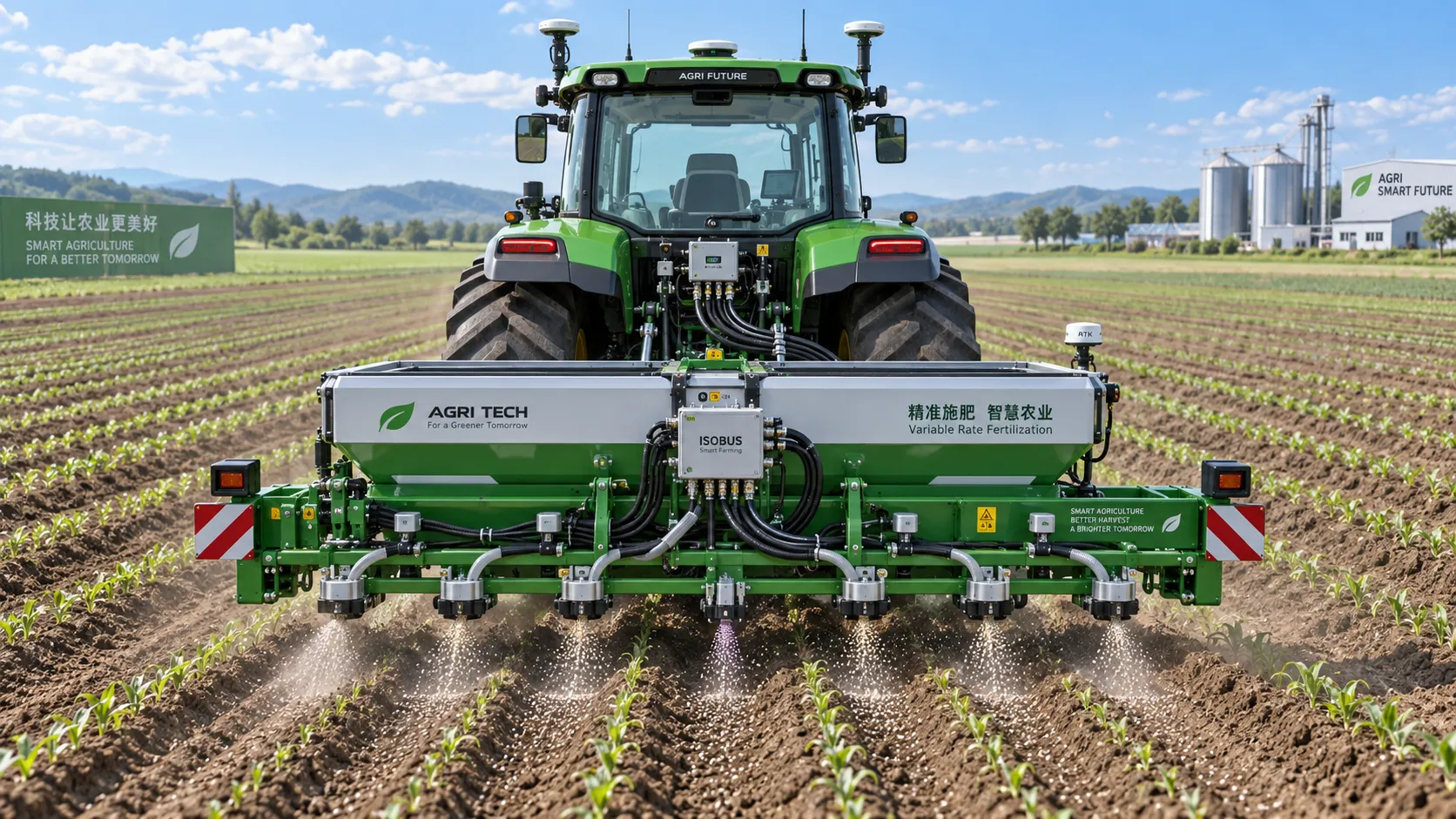
ISOBUS for Smart Agriculture: How It Connects Tractors, Implements, and Farm Data
ISOBUS for smart agriculture connects tractors, implements, terminals, and farm data—helping growers improve precision, documentation, and smarter field decisions.
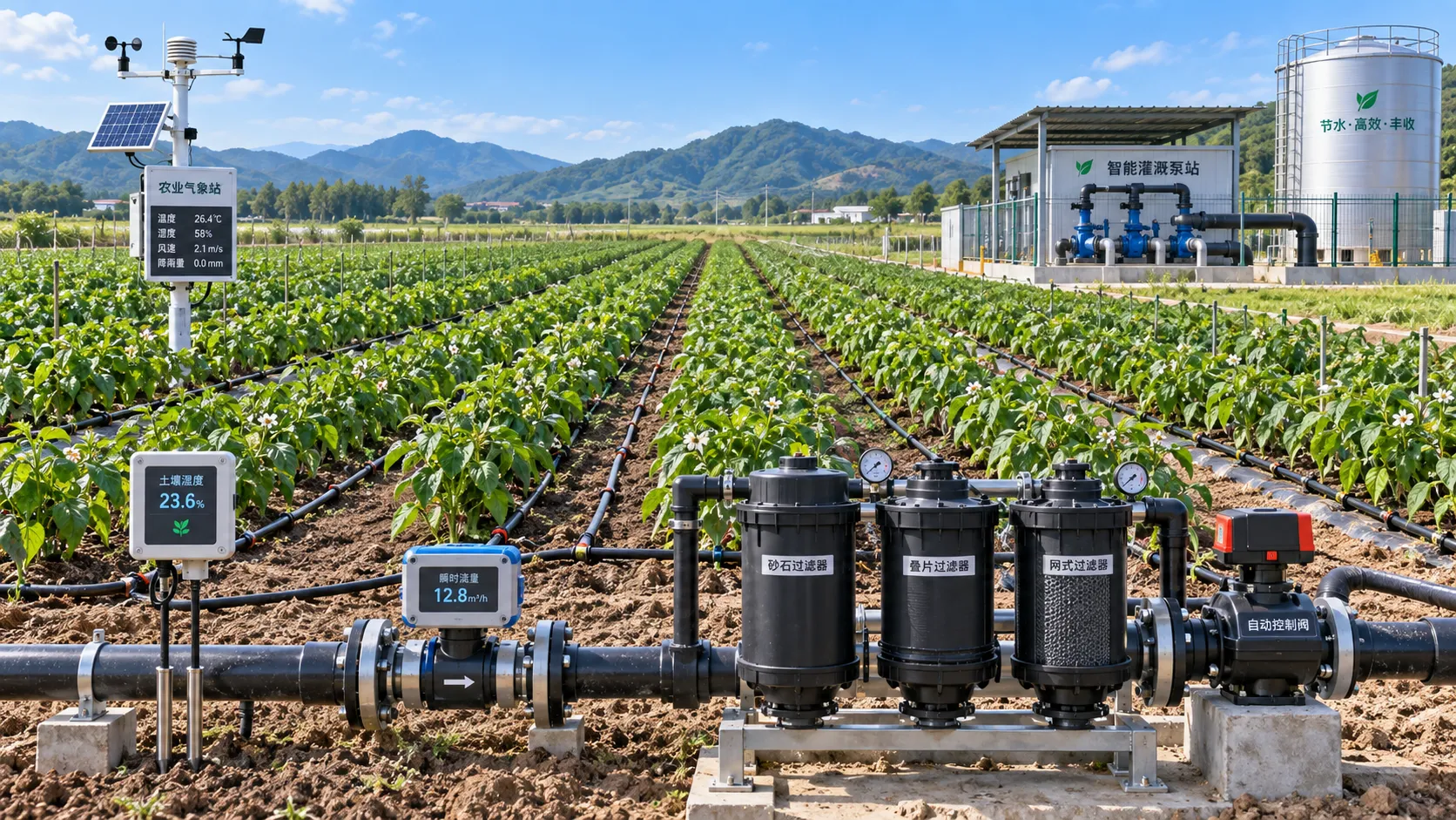
Automated Water-Saving Irrigation: How to Cut Water Use Without Reducing Crop Yields
Automated water-saving irrigation helps farms cut water use, protect crop yields, improve scheduling, and gain reliable control with sensors, flow monitoring, and smart zones.
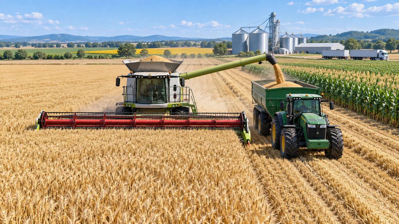
Selecting Grain Farm Equipment by Acreage, Crop Mix, and Harvest Window
Agricultural equipment selection for grain farming: match machinery to acreage, crop mix, and harvest windows to improve uptime, efficiency, and returns.
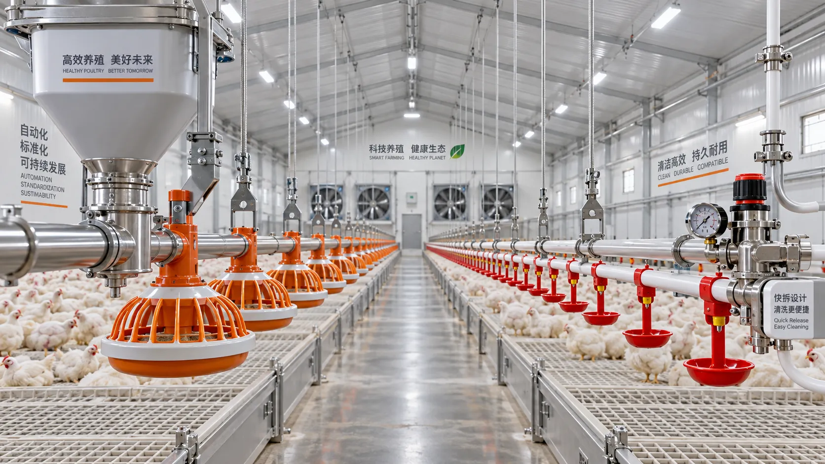
Poultry Equipment Selection: Evaluating Durability, Cleaning, and Compatibility
Poultry equipments selection guide: evaluate durability, cleaning access, and system compatibility to improve hygiene, reduce downtime, and support efficient flock management.
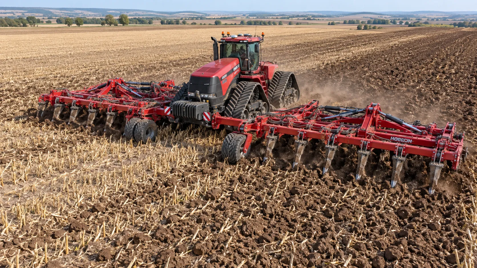
How to Select Heavy-Duty Farm Implements for High-Acreage, High-Horsepower Operations
Heavy duty farm implements: learn how to match draft, hydraulics, hitch capacity, frame strength, and field conditions for reliable high-acreage performance.
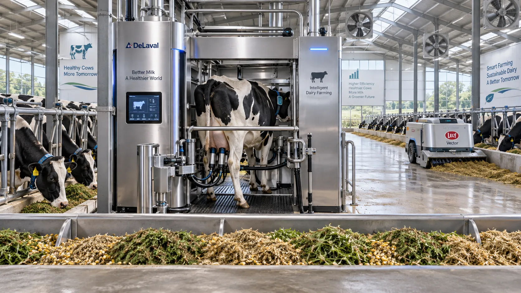
Smart Farming Technology for Dairy Farms: Where Automation Delivers Measurable ROI
Smart farming technology for dairy farms delivers measurable ROI through automation, precision feeding, health monitoring, and data-driven cost control.
Related News
- 00
0000-00
How Sensor Feedback Enables Accurate Variable-Rate Fertilization in Field Conditions - 00
0000-00
How to Select Precision Crop Protection Equipment for Variable Field Conditions - 00
0000-00
How to Evaluate Precision Fertilization System Suppliers for Farm-Scale Deployment - 00
0000-00
How to Select a Precision Fertilization System for Variable Corn Field Conditions - 00
0000-00
When does equipment for sustainable farming justify a higher capital spend?
Popular Tags
Tractor Power Architect
Weekly Insights
Stay ahead with our curated technology reports delivered every Monday.