Large-Scale Farm Equipment Cost Comparison: Price, Fuel, and Lifecycle Value
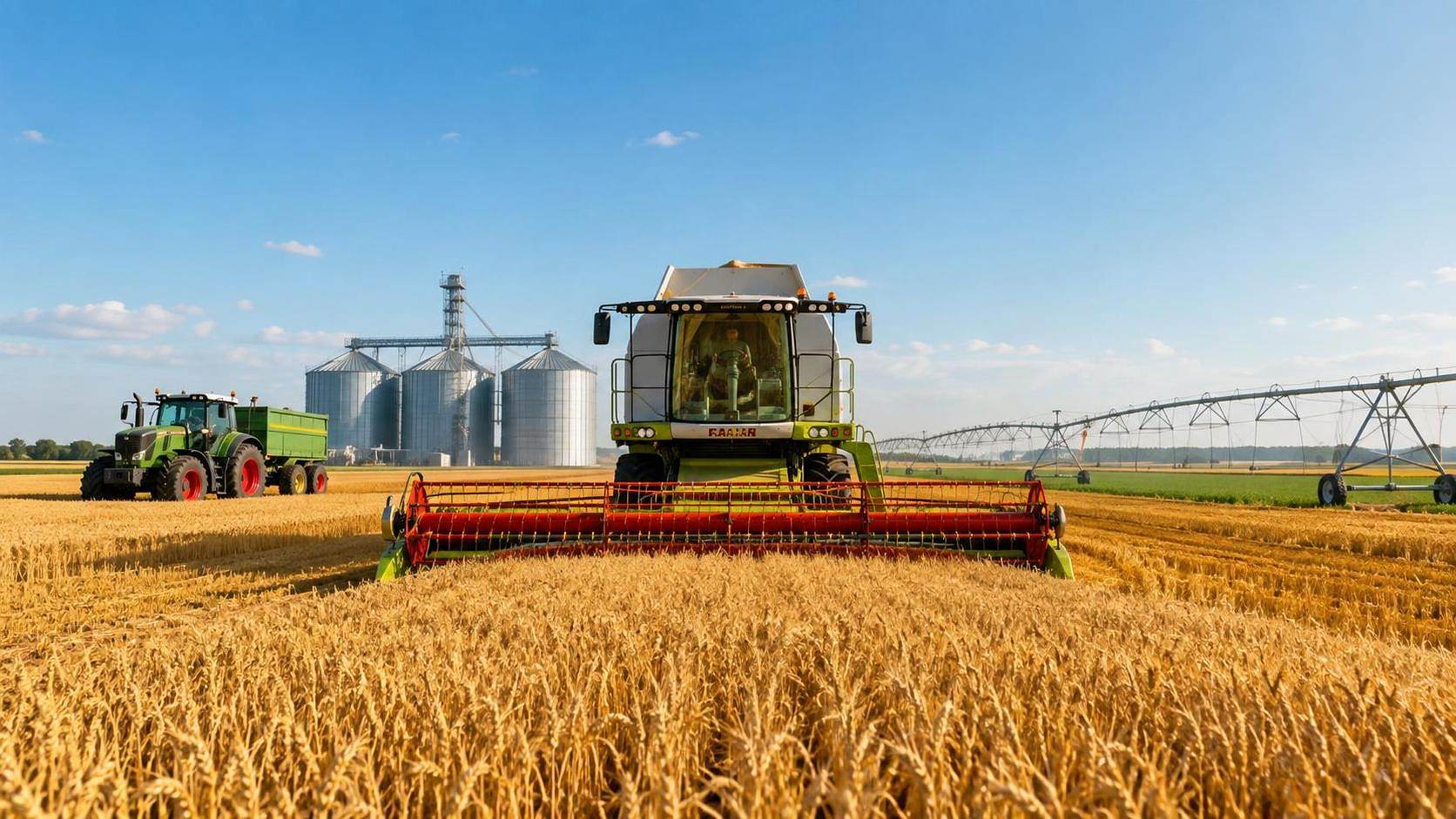




A large-scale farm equipment cost comparison is useful only when it explains how an asset consumes capital over its operating life. The purchase price is visible at the time of approval, but it is rarely the largest financial variable. Fuel, labor, maintenance, financing, depreciation, downtime, infrastructure requirements, and resale value can materially change the cost per hectare or cost per tonne of output.
The most economical machine is therefore not necessarily the one with the lowest quoted price. A higher-priced combine may produce a lower harvesting cost if it completes a narrow harvest window with fewer losses and less hired labor. A lower-cost tractor may become expensive if it lacks the hydraulic capacity, reliability, or annual utilization required by the farm. Likewise, an intelligent irrigation system should not be judged only by the price of controllers and emitters; its value depends on water availability, energy consumption, crop response, and the cost of managing a more complex system.
Purchase price is only the entry point
The initial invoice normally includes the base machine, selected attachments, transport, commissioning, taxes or duties where applicable, and sometimes training. Comparing only the headline quotation can create a misleading ranking between suppliers. One quotation may include a wider specification, while another may exclude essential implements, guidance hardware, spare parts, software subscriptions, or installation work.
A more useful comparison separates the initial investment into several categories:
- Acquisition cost: the machine, implements, options, delivery, and commissioning.
- Site and infrastructure cost: storage, workshops, electrical upgrades, fuel facilities, water distribution, or network connectivity.
- Operating cost: fuel, electricity, lubricants, consumables, labor, water, and routine service.
- Ownership cost: depreciation, insurance, financing charges, taxes, and the cost of capital.
- Risk cost: downtime, delayed field operations, crop losses, emergency repairs, and technology obsolescence.
The approval process should compare equivalent operating capability rather than equivalent invoice value. A tractor configured for heavy tillage, for example, should not be compared with a lighter unit without considering required work rates, traction, implement compatibility, and expected annual hours. The same principle applies to combines with different header widths, cleaning systems, grain tank capacities, or automation functions.
A practical lifecycle cost model
For a first-pass comparison, the annual ownership and operating cost can be represented as:
Annual total cost = depreciation + financing and capital cost + insurance and taxes + fuel or energy + maintenance and repairs + labor + consumables + downtime allowance
Cost per hectare or cost per tonne then depends on the useful annual output:
Unit cost = annual total cost ÷ productive hectares or tonnes completed
Depreciation should not be treated as an accounting item with no operational relevance. It represents the capital consumed while the machine is used. A simple estimate is the difference between acquisition cost and expected residual value, divided across the planned ownership period. The real pattern may be uneven: high-specification technology can lose value quickly if newer systems make older electronics or software unsupported, while durable mechanical components may retain value more steadily.
Financing also needs separate treatment. A machine with an attractive installment may still carry a substantial total interest burden, particularly when the repayment period extends beyond the period in which the asset generates its strongest productivity benefit. Approval should therefore consider both annual cash flow and total financing cost. Seasonal revenue patterns matter as well; a farm may earn most of its equipment-related income during a short harvest period while making repayments throughout the year.
Fuel efficiency must be linked to field output
Fuel consumption per hour is an incomplete measure. The more useful indicator is fuel cost per hectare, tonne, or completed operation. A tractor that consumes more fuel per hour but covers substantially more area may have a lower unit cost than a smaller machine operating near its capacity. Conversely, a high-horsepower tractor used for light work can create unnecessary fuel and depreciation expense through underutilization.
Fuel performance depends on load, soil condition, implement width, travel speed, tire setup, transmission strategy, operator behavior, and idle time. Official engine figures or supplier estimates should therefore be treated as reference points rather than guaranteed farm results. The comparison should use the duty cycle expected on the specific operation: deep tillage, planting, spraying, grain transport, or irrigation pumping have different load profiles.
Idle time deserves particular attention. Long warm-up periods, waiting for trailers, loading delays, field transfers, and bottlenecks at unloading points consume fuel without increasing productive output. Telematics can help identify these losses, but the financial benefit depends on whether the farm has the processes and personnel to act on the data. Paying for monitoring without changing utilization practices does not automatically reduce total cost.
For electrically powered equipment and irrigation systems, fuel cost is replaced by electricity demand, tariff structure, battery depreciation, charging infrastructure, and grid reliability. A lower energy price does not remove the need to evaluate peak-demand charges, backup power, and the cost of maintaining electrical equipment in dusty or humid environments.
Maintenance and downtime can outweigh small price differences
Routine maintenance is easier to budget than unexpected failure. Oil, filters, belts, bearings, tires, tracks, cutting components, hydraulic parts, and wear surfaces should be estimated according to operating hours and workload. Combines may incur particularly concentrated seasonal maintenance exposure because harvesting equipment operates under high dust loads and must be ready during a limited window.
Parts availability is a financial variable, not only a service issue. A machine with a lower maintenance schedule can still produce a higher lifecycle cost if critical components require long-distance shipping or specialized technicians. Import lead times, customs procedures, local dealer coverage, and the supplier’s parts stocking policy can influence the cost of an interruption.
Downtime should be modeled according to its consequence, not merely its duration. One day of delay during a flexible soil-preparation period is financially different from one day of delay during a short harvest window or a heat-sensitive irrigation period. For combines, delayed harvesting can increase field losses, grain moisture exposure, contractor costs, or the need to operate under less favorable conditions. The appropriate question is not “How reliable is the machine?” but “What financial exposure exists if this machine is unavailable at the critical time?”
Service agreements and extended warranties may reduce uncertainty, but they are not automatically economical. Their value depends on covered components, response times, exclusions, travel charges, labor rates, and whether the supplier can meet the required seasonal service window. A lower annual premium with weak response coverage may provide less protection than a more expensive agreement with enforceable parts and technician availability.
Tractors: capacity must match annual utilization
Tractor comparisons often focus on horsepower, but financial approval requires a broader capacity assessment. The relevant specification may include transmission type, hydraulic flow, lift capacity, ballast requirements, tire or track configuration, precision guidance compatibility, PTO capability, and the range of implements already owned.
A tractor is more likely to justify a higher capital cost when it replaces several operations, supports wider implements, reduces field passes, or keeps time-sensitive work within the available window. That benefit disappears if the farm lacks suitable implements, skilled operators, storage, or enough annual hours to spread fixed costs across output.
Over-specification creates a different problem. Excess power can increase purchase price, tire costs, fuel consumption, and financing exposure without improving work quality. Under-specification can cause low work rates, excessive wear, poor traction, and frequent operation at maximum load. The comparison should use the expected annual hours for each task and distinguish productive hours from transport, setup, and idle time.
Combine harvesters: throughput is valuable only when the system can absorb it
For combine harvesters, the purchase decision is tied to harvesting capacity and loss control. A larger machine may reduce the number of operating days, but its value depends on the availability of headers, grain carts, trucks, unloading capacity, operators, and suitable storage. If downstream logistics cannot absorb the combine’s output, the additional capacity may create waiting time rather than lower unit cost.
Harvest quality also belongs in the lifecycle calculation. Grain loss, damage, foreign material, moisture management, and cleaning performance can affect the saleable output and subsequent handling cost. These variables are influenced by crop type, yield conditions, terrain, operator settings, and weather, so they should not be converted into guaranteed savings without field-specific evidence.
Automation and machine monitoring can improve consistency and reduce adjustment errors, but software-enabled equipment introduces recurring costs and dependency on technical support. The financial case is stronger when the farm can use the data to improve settings, maintenance planning, route management, or operator performance. Otherwise, advanced functions may add capital cost without producing measurable operational gains.
Intelligent farm tools: separate measurable savings from capability
Precision planters, variable-rate applicators, guidance systems, and sensor-enabled tools can reduce overlap, improve input placement, or support more selective field operations. Their value is not determined by the presence of GPS, cameras, or sensors alone. It depends on field variability, data quality, prescription accuracy, compatibility with existing machinery, and the ability to convert recommendations into consistent action.
Financial assessment should include the complete digital stack: receivers, displays, correction services, software licenses, cellular connectivity, data management, calibration, and operator training. Compatibility is particularly important when equipment from different manufacturers must exchange maps, prescriptions, or machine data. A low-cost tool that cannot integrate with the existing fleet may require duplicate systems or manual data handling.
Input savings should be calculated conservatively. Reduced overlap may be easier to quantify than yield improvement, which is affected by weather, soil, crop genetics, and management quality. A sound approval model can assign different confidence levels to each benefit rather than combining every claimed advantage into one optimistic return estimate.
Irrigation systems have a different cost structure
Irrigation equipment combines capital expenditure with recurring energy, water, maintenance, and management costs. Pumps, pipes, filters, valves, controllers, emitters, sensors, power systems, and water storage may all be required. The financial comparison should account for installation and field layout, not only the price of individual components.
Energy consumption is influenced by pumping head, flow rate, pipe losses, pump efficiency, operating schedule, and water source. A system with efficient emitters can still perform poorly if pressure regulation is weak or filtration is inadequate. Maintenance costs may include flushing, filter cleaning, emitter replacement, pump service, leak detection, and sensor calibration.
Smart irrigation becomes financially relevant when it reduces unnecessary pumping, prevents overwatering, protects yield during critical crop stages, or lowers labor requirements for field inspection. Its return is harder to prove where water delivery is already tightly controlled or where field variability is limited. Connectivity and power resilience also matter: a highly automated system may need manual fallback procedures when communications or electrical supply fail.
How to compare competing quotations
Each supplier quotation should be converted into the same ownership scenario. Use the same evaluation period, annual operating hours, expected hectares or tonnes, financing assumptions, fuel or electricity prices, maintenance scope, residual value method, and downtime treatment. If assumptions differ, the result is a comparison of models rather than equipment.
A useful approval document should show at least three operating scenarios: expected utilization, lower utilization, and high-utilization or peak-demand conditions. This reveals whether the investment remains viable when acreage falls, fuel costs rise, harvest windows tighten, or maintenance costs exceed the base estimate. Sensitivity analysis is often more informative than a single return figure because equipment economics are highly dependent on utilization.
The strongest investment is the one that remains defensible under pressure
Large-scale farm equipment creates value when it converts capital into reliable productive capacity at an acceptable unit cost. The decision should therefore rest on operational output, not specification density or purchase-price discounts. A machine with advanced features may be financially sound when its functions reduce measurable losses, improve utilization, or protect time-sensitive production. It may be poor value when the farm cannot support the required infrastructure or lacks a clear method for measuring benefits.
The final comparison should present acquisition cost, annual cash requirement, lifecycle cost, unit cost, residual value, and downside exposure separately. Keeping these measures distinct prevents a low purchase price from concealing high operating risk and prevents an attractive productivity claim from masking weak utilization. For tractors, combines, intelligent tools, and irrigation systems alike, the approval question is straightforward: what output will the asset reliably deliver, what resources will it consume, and what financial exposure remains if assumptions prove wrong?
Related News
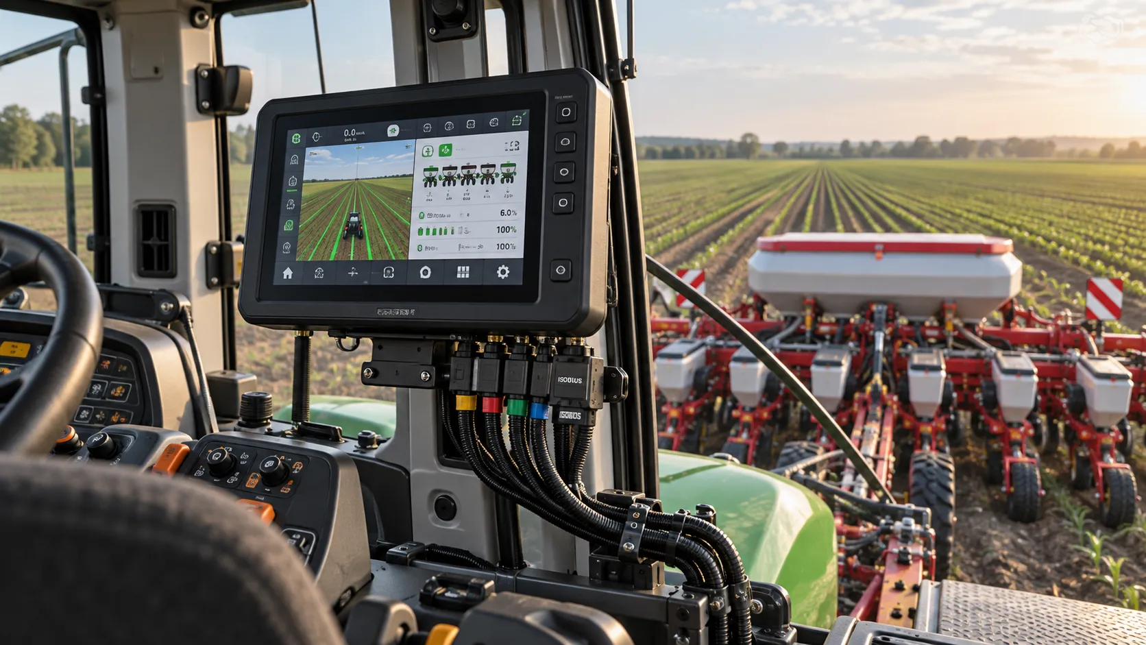
Choosing Precision Agriculture Controllers: ISOBUS and Variable-Rate Compatibility
Compare precision agriculture controllers for ISOBUS functionality, variable-rate compatibility, and data exchange. Discover what to test before buying to find the right fit for your fleet.
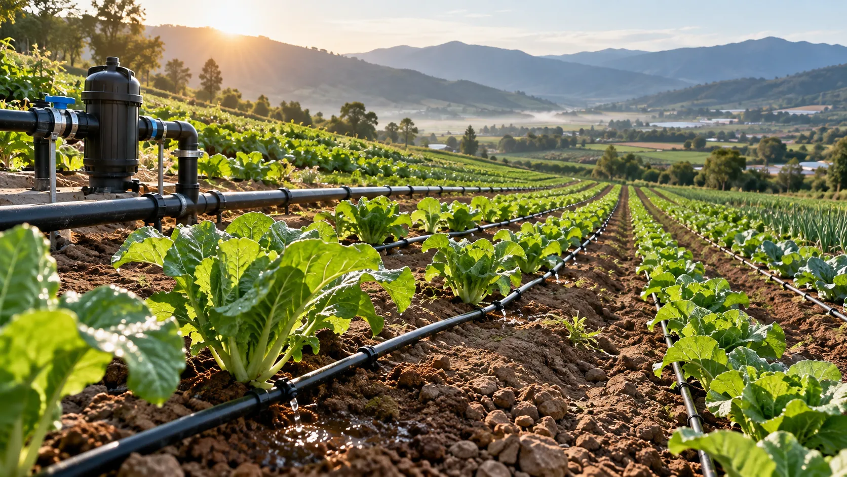
Choosing Drip Irrigation Systems for Open Fields: Soil, Slope, and Water Quality
Choose drip irrigation systems for open fields with confidence. Discover how soil, slope, and water quality shape emitter spacing, pressure, and filtration—and avoid costly design mistakes.
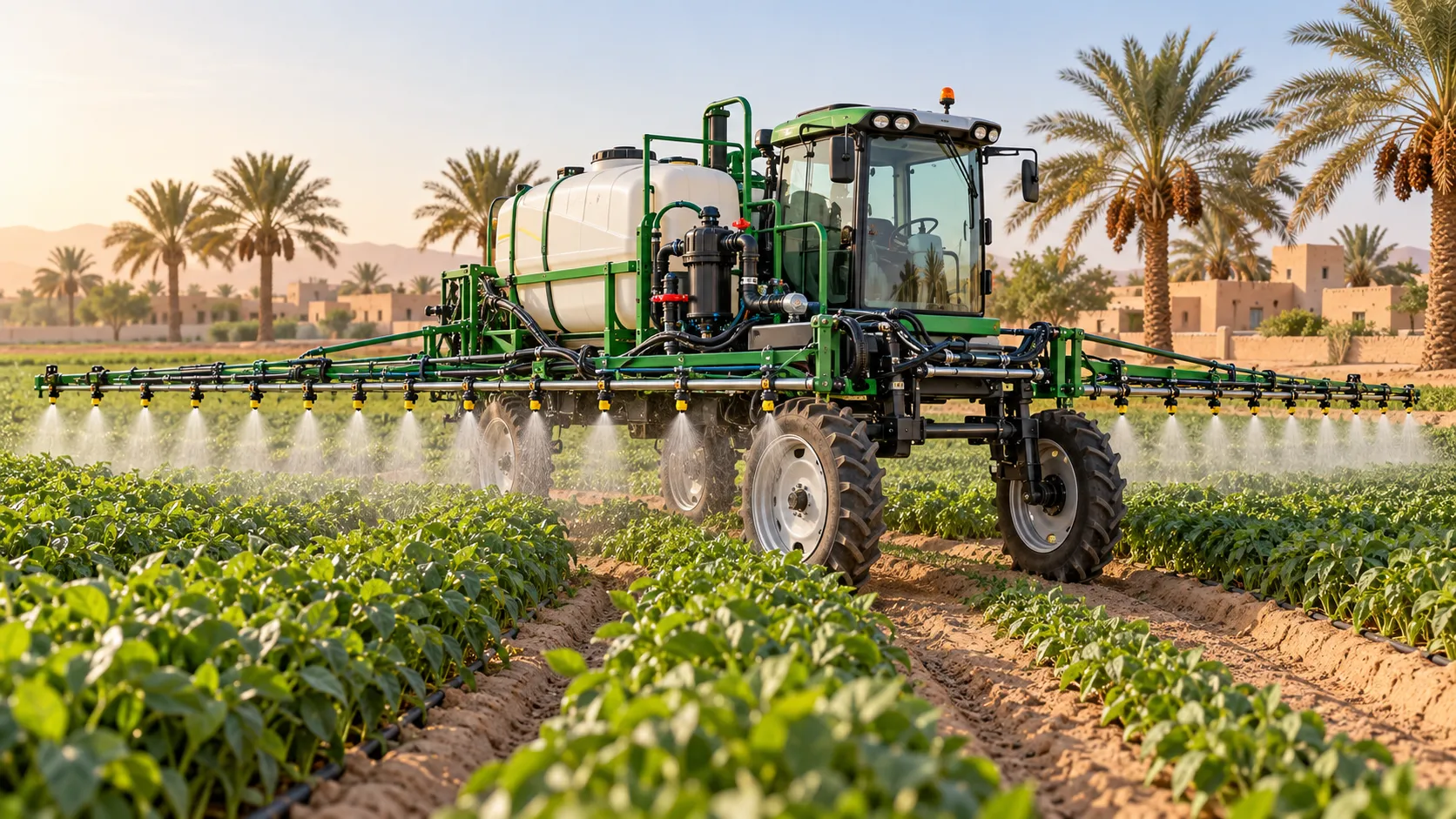
Choosing Crop Protection Equipment for Hot, Windy Middle Eastern Farms
Compare crop protection equipment Middle East farms need for hot, windy conditions. Discover key nozzle, drift-control, and durability checks to choose the right sprayer.
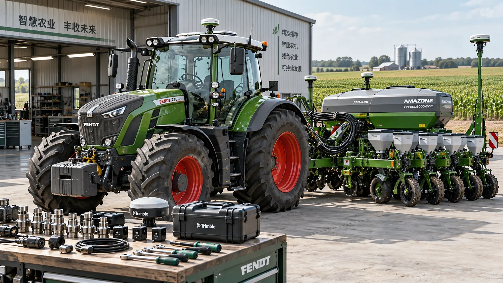
Choosing an Agriculture 4.0 Supplier: Compatibility, Support, and Total Cost
Choose an Agriculture 4.0 supplier with confidence. Learn how to verify compatibility, assess support, and compare total ownership costs to avoid hidden fees and costly downtime.
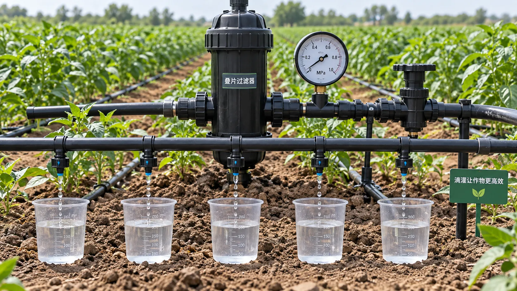
Low-Pressure Drip Irrigation: How to Fix Uneven Watering Without Raising Pressure
Optimize low pressure water-saving irrigation systems: discover how to fix uneven watering, clear blockages, and reduce hydraulic losses without raising supply pressure.
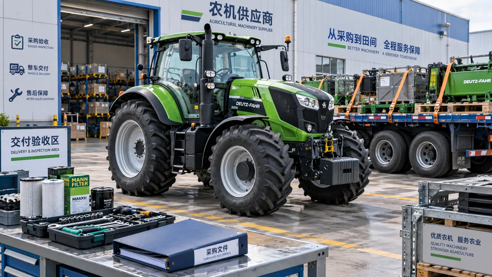
Comparing Farm Equipment Supplier Quotes: Price, Freight, and Warranty
Simplify supplier comparison for farm equipment price: assess freight, field-ready costs, and warranty coverage. Learn how to avoid hidden charges and choose a reliable supplier.
Choosing a Digital Farming Platform Provider: Compatibility and Data Ownership
Compare digital farming platforms providers on equipment compatibility, data ownership, and export rights. Discover practical checks to avoid lock-in and choose with confidence.
How Large-Scale Farm Telematics Cuts Downtime Across Mixed Fleets
Large-scale farm equipment telematics cuts mixed-fleet downtime with real-time alerts, smarter maintenance, and stronger operational control. Learn how to protect critical farm workflows.
How to Size Low-Pressure Water-Saving Irrigation Systems for Uneven Fields
Low pressure water-saving irrigation systems for uneven fields: learn zoning, pressure mapping, pipe sizing, and pump selection to improve uniformity and reduce water waste.
Related News
- 00
0000-00
Choosing Crop Protection Equipment for Hot, Windy Middle Eastern Farms - 00
0000-00
Choosing an Agriculture 4.0 Supplier: Compatibility, Support, and Total Cost - 00
0000-00
Comparing Farm Equipment Supplier Quotes: Price, Freight, and Warranty - 00
0000-00
Choosing a Digital Farming Platform Provider: Compatibility and Data Ownership - 00
0000-00
How Large-Scale Farm Telematics Cuts Downtime Across Mixed Fleets
Popular Tags
Ms. Elena Rodriguez
Weekly Insights
Stay ahead with our curated technology reports delivered every Monday.